Excel 2007 Data

In this tutorial we will be learning about the Excel 2007 data tab. This tab enables you to import data from other programs, update your spreadsheet when changes are made to the external data sources, sort, filter, and organize your data. Lets' get started with the first section, Get External Data.

 You can import spreadsheet information into Excel 2007 from about any program. Excel 2006 gives you a button to import from Access, a Web site, or Text file. Click one of those buttons and a window will open for you to select the location of the data you want to import.

If your data is in a source not listed click the down arrow on From Other Sources and make a selection. If you need help please email me and I will walk you through your specific question. The last button is Existing Connections. The benefit of using a data source connection is it can make it less time consuming to analyze data in Excel from other programs. Usually you would have to cut and paste data into Excel with the Data Source connections you don't have to do that.

 Let's Move on to the Connections section of the data tab. The first button is Refresh All. If you have your spreadsheet connected to a data source and you make changes to your data source then you will need to update your spreadsheet. Click the Refresh button you will be given the option to update all data sources, update just the work book, check on the status of the refresh, or cancel the refresh.

The Connections button will open a window that gives you a list of all of your data connections a description of the connection, where the connection is located and the last time it was refreshed.
The Properties button will be grayed out until you have a data source connected to your spreadsheet. Properties with tell you how cells that are connected to a data source will be updated, what contents from the source will be displayed, and how changes in the number of rows or columns in the data source will be handled in the workbook.

The Edit Links button will open a window for you to view all other files the spreadsheet is linked to and how they are linked and it will allow you to make changes to the links.

 The next section is Sort & Filter. If you have large amounts of data in your spreadsheet it is helpful to be able to organize it and find what you are looking for. To use any of the sort buttons you can click the top of the column or highlight all of the data you want sorted then click the button you would like to organize your data with. The AZ button with the down arrow will sort your data from lowest to highest. The ZA button with the up arrow will sort your data from highest to lowest.

 The Sort button opens the Sort window which will give you more options when organizing your data. You can sort on multiple levels if you have several columns of data. For example you could sort my last name, then date, then amount owed. Make you selections then click the OK button to finish and your data will be sorted.

To use the filter button select the cell at the top of the column you want to filter then click the filter button. This will place an arrow in the cell. When you click the down arrow you will get a menu to make your filtering selections.

In this example I am filtering a date column. It gives me the option to just show 2010 dates, all dates, etc. You can either check the boxes provided to filter or click the Date Filters option to have more choices such as filter by quarter, month dates past today, etc. Play with the options and when you are finished click ok for the filter to take place. To clear a filter click on the down arrow and select Clear filter From "column name" or click on the clear filter from the sort and filter section of the data tab.


The last button in the sort and filter section is the Advanced tab. This will open a window for you to customize your filtering more.

Next is the Data Tools section. The first button is Text to Columns. This button will separate words into 2 columns.

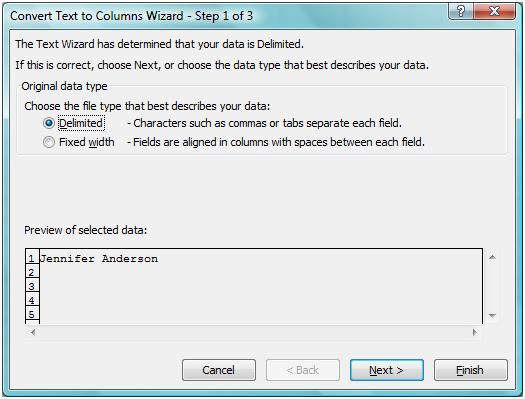
To try this type you first and last name in one cell. Then click the Text to Columns button. It will open the Convert Text to Columns Wizard.

 The first step of the wizard has you tell Excel how your words are separated in the cell. I need to click Fixed width because I just used a space. Then click next. In the next window lets you set the column widths. You can adjust the widths by moving the arrows. When finished click next for the third window. The third window has you set the type of cell format, ie: text, currency, etc. make your selection and click finish. It will return you to your spreadsheet with all of the selected cells separated into 2 cells.